Once you've updated the set_path variable, you can run the script. This will input the data, generate the HGM, and create the confusion matrices all in one script.
Part 1B: HGM Generation
Understanding Wetlands Classification Systems
Cowardin System
The Cowardin classification system includes five classes: riverine, lacustrine, palustrine, marine, and estuarine (FGDC, 2013). NWI is the largest database of geospatial wetlands data within the United States and uses the Cowardin classification. This tutorial uses NWI as the data source for the Cowardin classed wetlands. Using NWI, three wetland types are found within the study area: 566,902 acres of palustrine (44.3%), 217,458 acres of riverine (17.0%), and 68,720 acres of lacustrine (5.4%) wetlands. Wetlands dominate the study area, covering about 67% of the landscape.
Note: As part of data pre-processing, the NWI data was modified to remove open water from the classification in order to make the data comparable to the HGM system, which does not account for open water.
HGM System
The HGM classification system includes seven classes reflecting landscape functionality: riverine, depressional, slope, mineral soil flats, organic soil flats, tidal fringe, and lacustrine fringe (Smith et al., 2013). In order to be comparable with the Cowardin system, the HGM classification was modified into three classes matching the Cowardin classes present within the study area (riverine, lacustrine, and palustrine). Riverine and lacustrine classes exist within both classification systems; however, the palustrine class is only in the Cowardin system. To better align the two systems a “palustrine” class was created for the HGM by combining depressional, slope wetlands, mineral soil flats, and organic soil flats definitions. The HGM palustrine class describes wetlands whose main water sources are groundwater or precipitation rather than flows from rivers or lakes. No geospatial layers using the HGM exist for this study area, so a wetlands database was created using ancillary data and the modified HGM classification system. This process is described below, and there are published examples of research that used GIS data to create an HGM dataset (Cedfeldt et al., 2000; Adamus et al., 2010; Van Deventer et al., 2016; Rivers-Moore et al., 2020).
In addition to inputting the data, the script you just ran also generates the HGM dataset. In order to do so, the code uses ancillary data including hydrogrophy, hydric soils, and elvation layers. All rivers and lakes larger than eight hectares are given a 30m buffer and then areas within this buffer with either hydric, predominantlyhydric, or partially hydric soils are classed as riverine. Areas adjacent to lakes with hydric, predominately hydric, or partially hydric soil are classed as lacustrine. Elevation is used to locate topographic depressions and slopes reater than two percent with hydric, predominately hydric, or partially hydric soils - classed as palustrine along with areas that had completely hydric soils.
The HGM dataset was intended for comparability with NWI. It was not created with the goal to be a more accurate wetlands model. Several assumptions were made in generating the HGM dataset that may not be true in every geographic case. For example, it is not correct to assume that soils classed as hydric are always wetlands, or that wetlands adjacent to rivers and lakes are always riverine and lacustrine respectively. Wetland classification is more nuanced and requires on-the-ground validation for the highest accuracy. However, the purpose of this analysis is to demonstrate a method and data framework within which to explore multi-scale patterns of spatial uncertainty, rather than to establish a spatially precise model of wetlands within the study area.
Part 1C: Confusion Matrices
Understanding Confusion Matrices
Here we are using confusion matrices to compare the NWI and HGM wetlands classes. We are using the NWI data as the validation dataset and the HGM as the test dataset; this is not to imply that the NWI dataset is more or less reliable than the HGM dataset. Both wetland datasets incur uncertainties resulting from their compilation, processing, and temporal resolution. The confusion matrices simply allow us to identify the agreement and disagreement between the two datasets. Where the two wetland classification systems agree, we have higher certainty that the classification of the wetland presence or type is reliable. Conversely, where there is disagreement, there is higher uncertainty.
Understanding Evaluation Metrics
Within the confusion matrices, there are three evaluation metrics used to quantify uncertainty: Recall, Precision, and F1.
- Recall defines the ratio of true positives to real positives (true positives + false negatives), measuring how often the HGM data agrees with an NWI positive classifications of wetlands presence or type. This metric ranges from 0 to 1, with lower numbers indicating areas of more disagreement.
- Precision defines the rate of true positives over predicted positives (true positives + false positives), measuring how often the NWI data agrees with and HGM positive classification of wetland presence or type. Like Recall, this metric ranges from 0 to 1, with more disagreement yielding lower scores.
- F1 is the weighted harmonic mean of Recall and Precision, measuring the rate of disagreement between the two classification systems. Where HGM and NWI agree, we will have an F1 score of 1. (Powers, 2011)
Generating and Mapping Confusion Matrices
To check your outputs, navigate into your Part 1 Output folder and open up the Full_Keys.xlsx which contains both your coarse and fine confusion matrices. The first tab in the excel contains your coarse confusion matrix and should look like this:
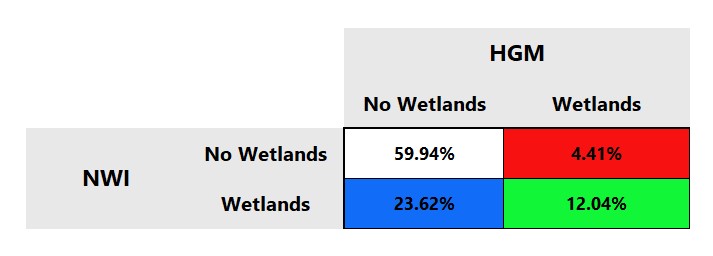
This coarse resolution assesses the presence versus absence of wetlands. This matrix is shows that we have 12.04% true positives (green) in our study area and 59.94% true negatives (white) - both refer to areas where NWI and HGM agree on the presence or absence of wetlands. We also have 4.41% false positives (red) and 23.62% false negatives (blue) - both referring to areas where NWI and HGM disagree. Since these matrices use NWI as the validation dataset, false positives are areas where the NWI classifies a wetland while HGM does not and false negatives are areas where the NWI classifies no wetlands while HGM classifies the presence of wetlands.
The second tab in your excel contains the fine resolution matrix and should look like this:
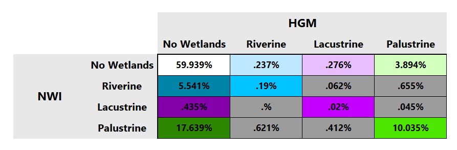
This fine resolution confusion matrix compares not only the presence and absence of wetlands, but also the agreement of the specific wetlands type (riverine, lacustrine, or palustrine). The first column shows false negatives (wetlands in NWI but not in HGM) for all categories while the top row shows false positives (wetlands in HGM but not in NWI). The diagonal shows cells that agree on the presence/absence of wetlands in both data sets as well as on their specific type. The six gray cells indicate a misclassification at the finer level, namely that both classification systems agree that wetlands are present but disagree on the type. The percentage values in the matrix indicate the proportion of the pixels in each of the sixteen cases for the entire study area. The cells are color-coded, with hue (blue, green, purple) referring to wetland type. Saturation and value are used to distinguish false negatives and false positives.
Other outputs from Part 1 include:
- CoarseAttributes_Full.csv
- This give the count of pixels and percent of the study area that fall into true negatives, false negatives, true positives, and false positives at the coarse attribute uncertainty level.
- CoarseStats_Full.csv
- This provides the Recall, Precision, and F1 scores for the study area at the coarse level of analysis.
- FineAttributes_Full.csv
- Need info from Kate on what/how the IDs correspond to
- FineStats_Full.csv
- Need info from Kate on how to explain the multiple scores This provides the Recall, Precision, and F1 scores for the study area at the corase level of analysis.
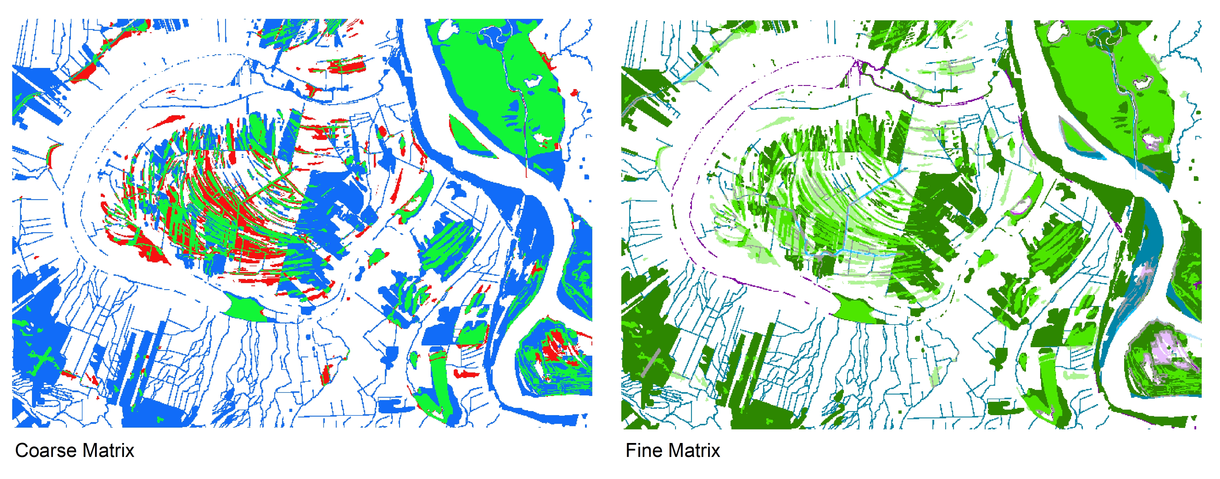
- coarse_matrix.tif and fine_matrix.tif
- These both allow you to visualize the categories from the confusion matrices across the study area using ArcMap or QGIS; see instructions below. Note that if you simply open the tifs in a photo viewer, they will look completely black, but if you follow the steps below you can visualize the confusion matrices.
- Scratch outputs within the Part1/Data/Scratch folder
- These are intermediary outputs. You don't need these, but if you want to explore more or adopt this tutorial to your own data these scratch outputs can be useful to identify patterns or isolate intermediary processes.
Mapping the Confusion Matrices in ArcGIS
- Open ArcMap and load in coarse_matrix.tif
- Open up the properties of the course_matrix layer and go to the Symbology tab.
- On the left side of the Properties window, click 'Unique Values'.
- A message will pop up saying 'Raster attribute table doesn't exist. Do you want to build attribute table?'
- Click 'Yes'.
- Towards the bottom left of the Properties window, clik on the 'Colormap' button. A dropdown will appear, click on 'Import a colormap...'
- OIn the file explorer window that pops up, navigate to Part1>Output>Colormaps. Within the Colormaps folder, double click on Coarse Surface colors.clr.
- Click 'OK' to apply your changes and close the Properties window. You'll notice that the colors used correspond to the colors of your confusion matrix in Full_Keys.xlsx.
- To map at the fine resolution repeat the steps above, using fine_matrix.tif and Fine Surface Colors.clr.
Note: These instructions were made using ArcMap 10.8
Mapping the Confusion Martrices in QGIS
- Open up QGIS and loas in coarse_matrix.tif
- Open up the layer properties of coarse_matrix and go to symbology.
- Under 'Render type' change dropdown selection to 'Paletted/Unique values', then click the 'Classify' button. You should see the values '0', '1', '10', and '11' pop up.
- Change the colors to match the confusion matrix. Double click each color chip and change the HTML notation in the 'Select color' window that pops up. Then click 'OK' to move on to the next color.
- Change the color chip for '0' to white (#FFFFFF).
- Change the color chip for '1' to blue (#116DF7).
- Change the color chip for '10' to red (#F71111).
- Change the color chip for '11' to green (#11F737).
- Once you've changed all the colors, click 'Apply' to apply your changes and 'OK' to close the layer properties window.
- You have now mapped the coarse confusion matrix in GQIS!
- To map the fine matrix follow the steps above using the fine_matrix.tif and the following colors:
- '0' - white (#FFFFFF)
- '1' - dark blue (#0084A8)
- '2' - dark purple (#8400A8)
- '3' - dark green (#2D8700)
- '10' - light blue (#BEE8FF)
- '11' - medium blue (#00C3FF)
- '13', '21', '23', '31', and '32' - all gray (#9C9C9C)
- '20' - light purple (#E8BEFF)
- '22' - medium purple (#C300FF)
- '30' - light green (#D3FFBE)
- '33' - medium green (#4CE600)
Note: These instructions were made using QGIS 3.16